The 5-Step Guided Workflow
Every Vizalyze project follows the same ribbon-based flow. Each step is accessible at any time - click the ribbon button to jump directly. The app keeps state across steps and highlights the active phase.
| Step | What it does | Key outputs |
|---|---|---|
| 1 · Load | Import files, decode CAN/LIN, apply templates, preview before loading | Loaded dataset, Parquet cache, channel list |
| 2 · Health | Automatic data quality check with actionable recommendations | Pass/Warn/Fail badge, completeness score, issue list |
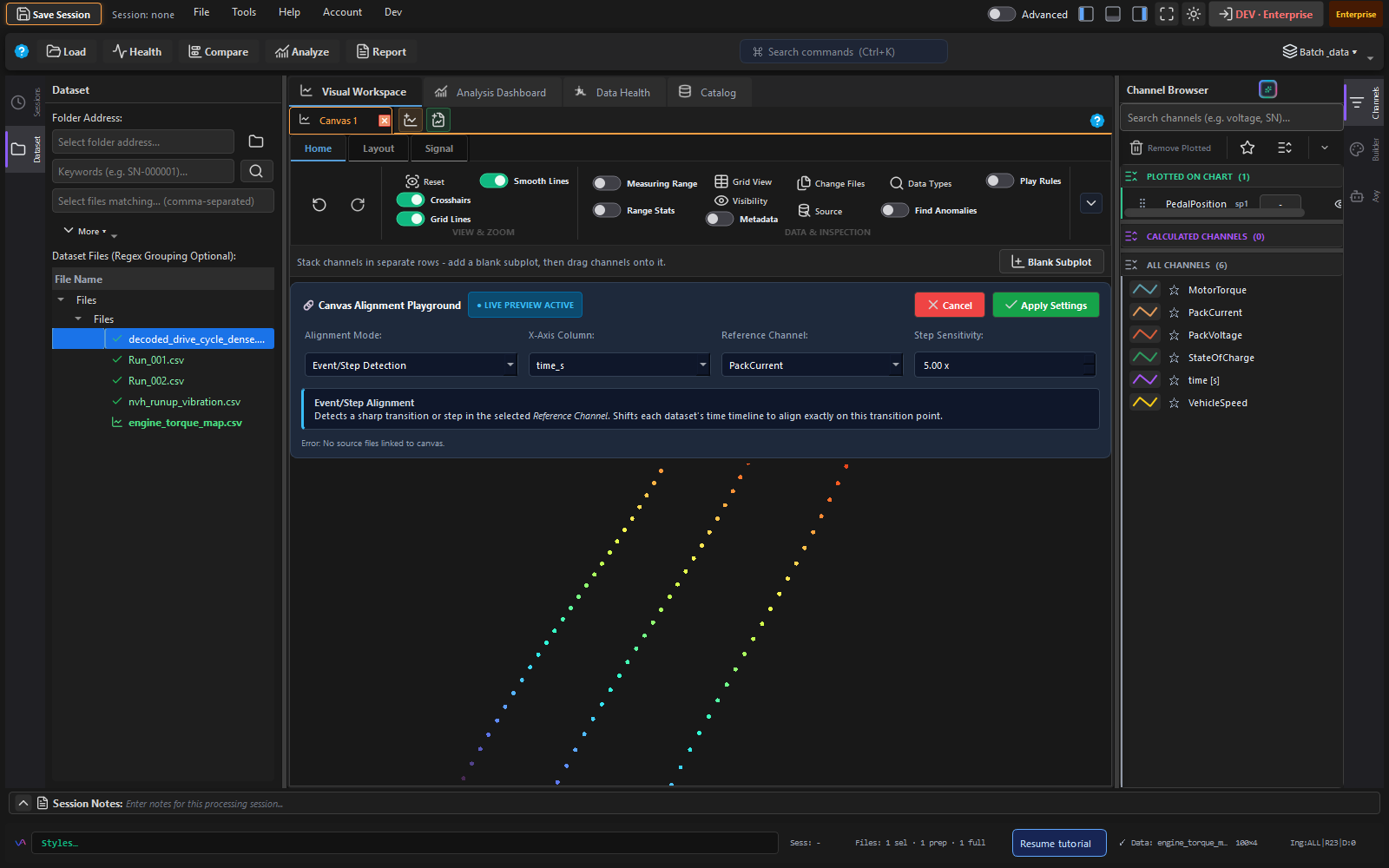
| 3 · Compare | Overlay multiple runs with 6 alignment modes, delta tables | Overlaid chart, delta table, lineage entries |
| 4 · Analyze | Statistics, correlations, KPIs, limit evaluation per domain profile | Stats table, correlation matrix, limit badges |
| 5 · Report | Batch export to PPTX/Word/PDF from reusable templates | Report files, pipeline recipe JSON |
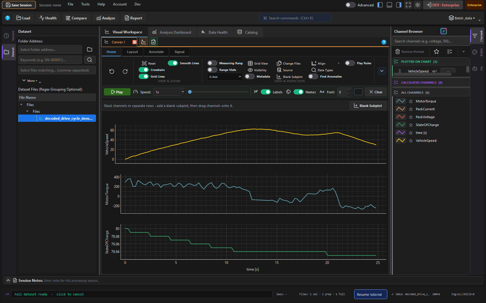
Load & Import
Vizalyze's import engine handles 31+ file formats with intelligent preamble detection, unit extraction, CAN bus decoding, locale-aware decimal/date parsing, and lazy loading for fast previews on large files.
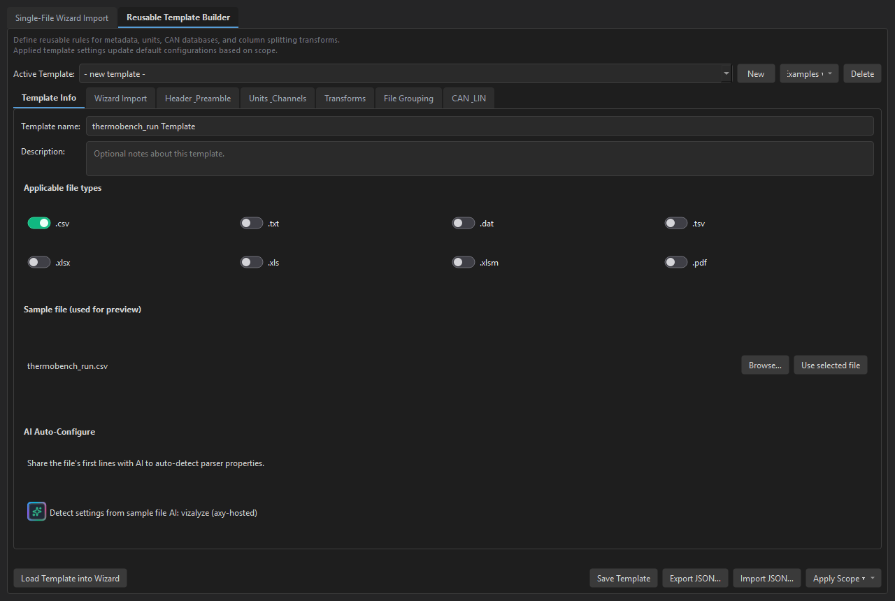
Import Template Builder
Create reusable import configurations from Tools → Data → Import Template Builder. Templates capture:
- Preamble parsing rules (rows, regex, delimiter modes)
- Header-row detection and unit extraction (metadata vs row-based)
- Channel cleanup rules (regex replacements, per format)
- File-grouping rules and CAN/LIN database assignments
Templates are saved as JSON in Import_Templates/ and can be applied per-file, per extension, or as a global default. Share templates across machines by exporting the JSON.
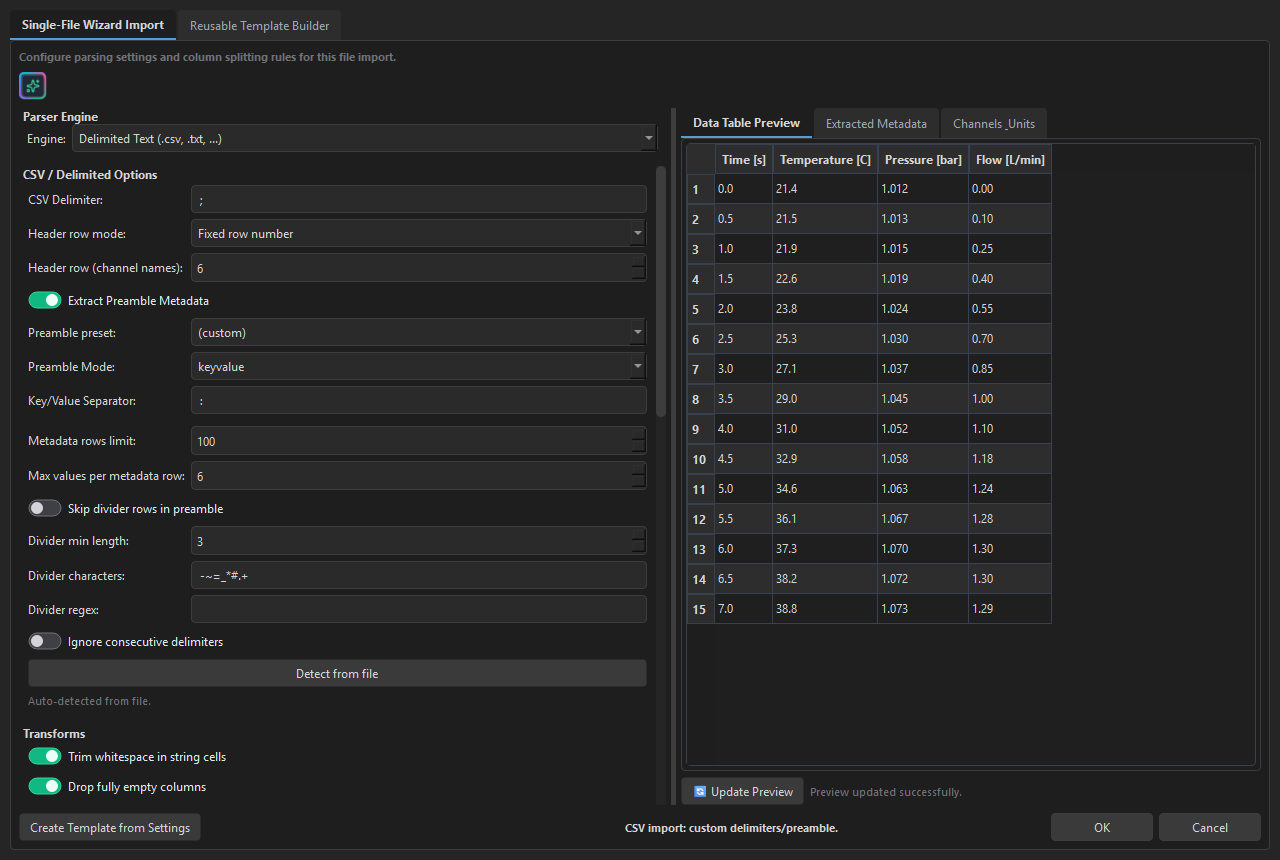
Advanced Import Utility
Open from Tools → Data → Advanced Import Utility for per-file import tuning without saving a template - preamble modes, delimiter detection, column cleanup, and live preview on messy lab exports.
Preamble Parsing
Many test data files contain header metadata before the actual data table. Vizalyze auto-detects the header row and offers 5 preamble modes:
- Auto - automatically detects format (recommended)
- Key-value - parses
Key: Valuepairs - Delimited - fixed delimiter (comma, semicolon, tab)
- Regex - custom pattern per line
- Raw - skip N rows, take the rest as-is
Vendor Format Auto-Detection
Vizalyze uses a two-pass content sniffer to identify file formats from their actual bytes, independent of file extension. This handles mislabelled files, non-standard extensions, and vendor exports that look like plain CSV or binary blobs.
- Pass 1 - Binary magic bytes: HDF5, Apache Parquet, Arrow/Feather, SQLite, PDF, Excel OLE2/OOXML, MATLAB workspace, ASAM MDF, Vector BLF, NI TDMS
- Pass 2 - Text header fingerprints: Gamry Framework DTA (
EXPLAINheader), Zahner Zennium / IM6 EIS data, Bronkhorst FlowView, Siemens WinCC / SIMATIC, Mettler-Toledo LabX, Metrohm MagIC Net, Dewesoft ASCII export, NI LabVIEW LVM
When the sniffer detects a format with high or medium confidence, the loader routes to the correct parser and the Advanced Import wizard pre-fills delimiter, mode, and vendor hints automatically.
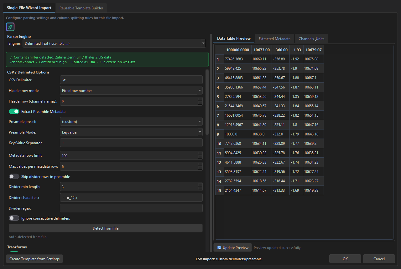
data.txt is identified as Zahner Zennium EIS data - delimiter and preamble hints are pre-filled and the preview shows the impedance table.Excel & PDF Import
For Excel files: configure sheet policy (first / all / prompt), and use the range suffix syntax file.xlsx:::SheetName:::B5:Z5000 for precise cell ranges.
For PDF files: Vizalyze uses pdfplumber to extract tables. A region picker dialog lets you select the exact table area on the page.
Lazy Loading & Performance
Large CSV files are previewed using Polars scan_csv() (lazy evaluation) - only the first 2,000 rows load for the preview. Full load happens on demand. Loaded files are automatically cached as Parquet for near-instant re-open.
Data Health Panel
The Health panel runs an automatic quality audit on every loaded dataset and produces a compact, actionable summary. It's the first thing to check after loading new data.
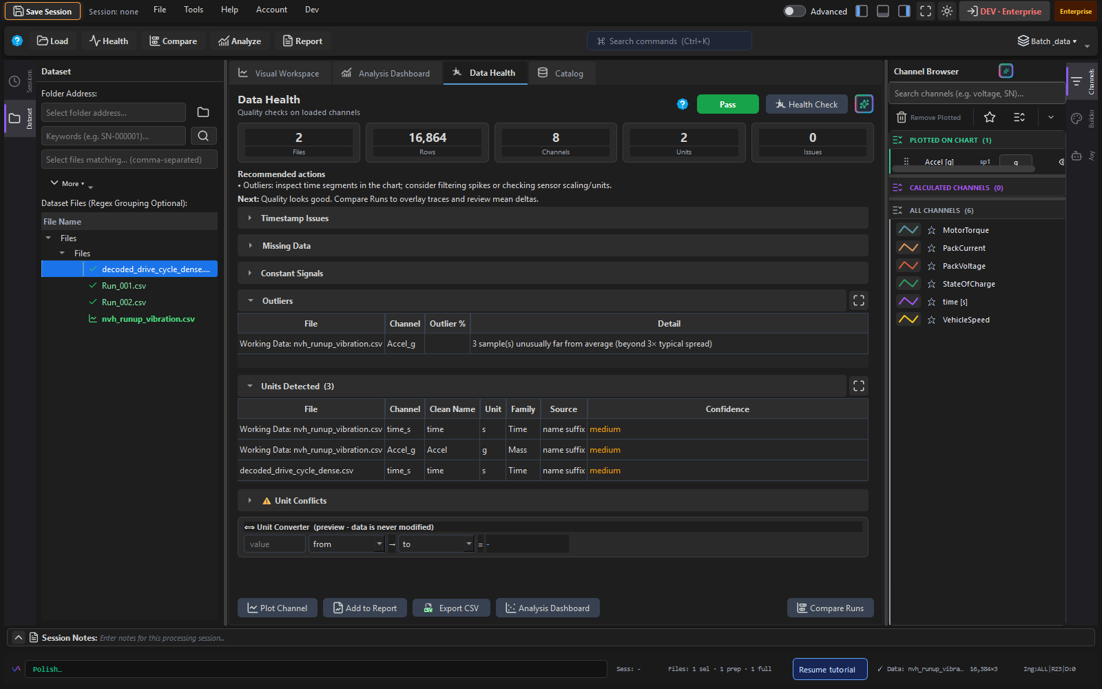
What it checks
- Data completeness - percentage of non-null values per channel
- Constant channels - channels with zero variance flagged as potential sensor faults
- Timestamp conflicts - monotonicity checks, duplicate timestamps, irregular intervals
- Unit consistency - detects channels in different unit families mixed together
- Sampling rate - estimated from time column, checked for consistency
Status badges
Each channel gets a badge. The overall dataset badge is the worst of all channels. Clicking a badge jumps to the recommended fix in the Compare or Analysis panel.
Recommended actions
The panel maps each issue to a concrete next step - e.g., "3 channels have >5% missing data → open Compare Runs and enable interpolation" or "Timestamp duplicates detected → use step alignment mode".
Compare Runs
Overlay any combination of loaded datasets on a single chart, automatically aligned to a common time base. Works across different file formats and sampling rates.
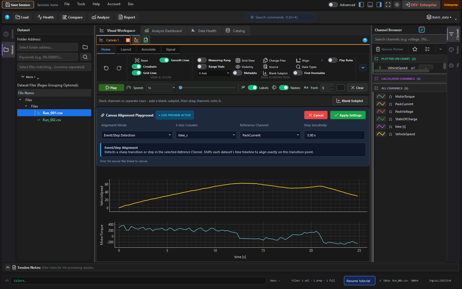
Alignment modes
| Mode | Best for |
|---|---|
| Time column | Runs with identical absolute timestamps (e.g., same test bench clock) |
| Uniform resample | Runs at different sampling rates - linearly interpolated to a common grid |
| Event / step | Marker-based alignment to a named event in each run |
| Setpoint crossing | Align on when a channel first crosses a threshold value |
| Trend t=0 | Zero time at the start of each run (relative alignment) |
| Row index | No time column - align by row number |
Delta table
Switch to Delta Table view to see the numerical difference between runs for every channel. Shows mean, max deviation, and a pass/fail indicator against user-set tolerances.
Y-offset tools
Per-run Y-offset: zero at min, max, mean, start, or end of each channel. Useful for removing DC offset before shape comparison.
Missing channel warnings
If a channel exists in some runs but not others, the panel shows a warning with options to skip, fill with NaN, or use a default value.
Analysis Panel
Go beyond charts with computed statistics, correlation matrices, domain KPIs, and limit evaluation - all driven by 8 selectable domain profiles.
Statistics
Per-channel: min, max, mean, std, median, P5, P95, skewness, kurtosis. Supports up to 240 channels and 200k rows in a single analysis. Export to CSV or directly into the report template.
Correlation analysis
Pearson correlation matrix for up to 16 channels at once. Highlights strong positive/negative correlations above a configurable threshold. Useful for identifying redundant sensors or causal relationships.
Domain profiles
Select a domain profile to get pre-loaded KPI recommendations, suggested analysis sections, and appropriate limit defaults:
- Generic - universal statistics, no domain assumptions
- Fuel Cell - stack voltage, current density, power density, efficiency KPIs
- Battery - SOC, capacity, C-rate, temperature gradient KPIs
- Thermal - heat flux, temperature uniformity, thermal resistance
- Vehicle - acceleration, braking, energy consumption per km
- Emissions - NOx, CO, HC, PM cycle-averaged values
- Pharma HPLC - retention time, peak area, resolution, tailing factor
- Pharma GC / MS - TIC, BPI, spectral purity, fragment ion ratios
Limit evaluation
Define upper/lower limits per channel. The analysis panel evaluates each channel against its limits and assigns Pass / Warn / Fail badges. Limit definitions can be saved to recipes for reuse.
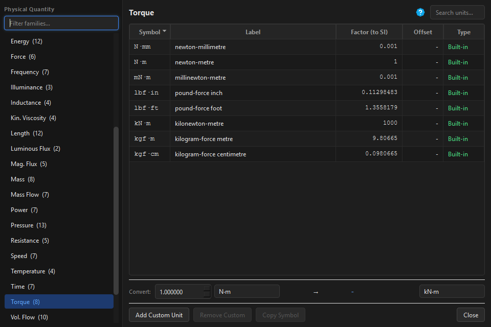
Unit detection & conversion
The Units tab detects engineering units from channel names and metadata, then suggests affine conversions so channels can be compared fairly. The full Unit Library (Tools → Units → Engineering Unit Library) covers 30+ families and 200+ built-in units.
Batch Reporting
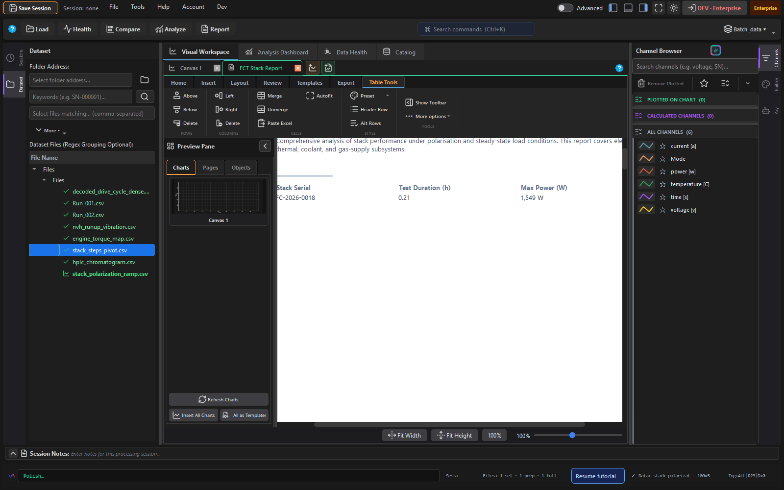
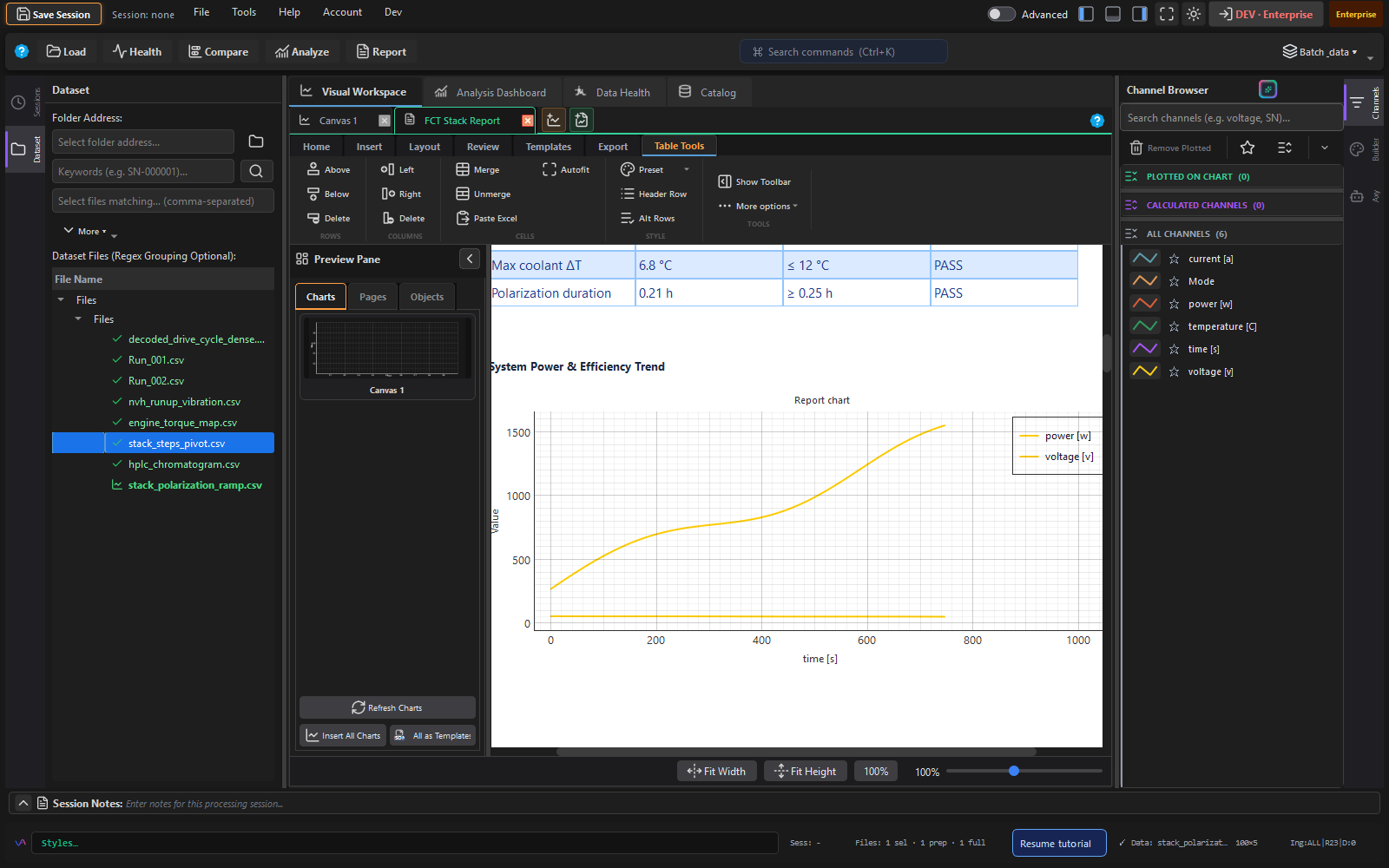
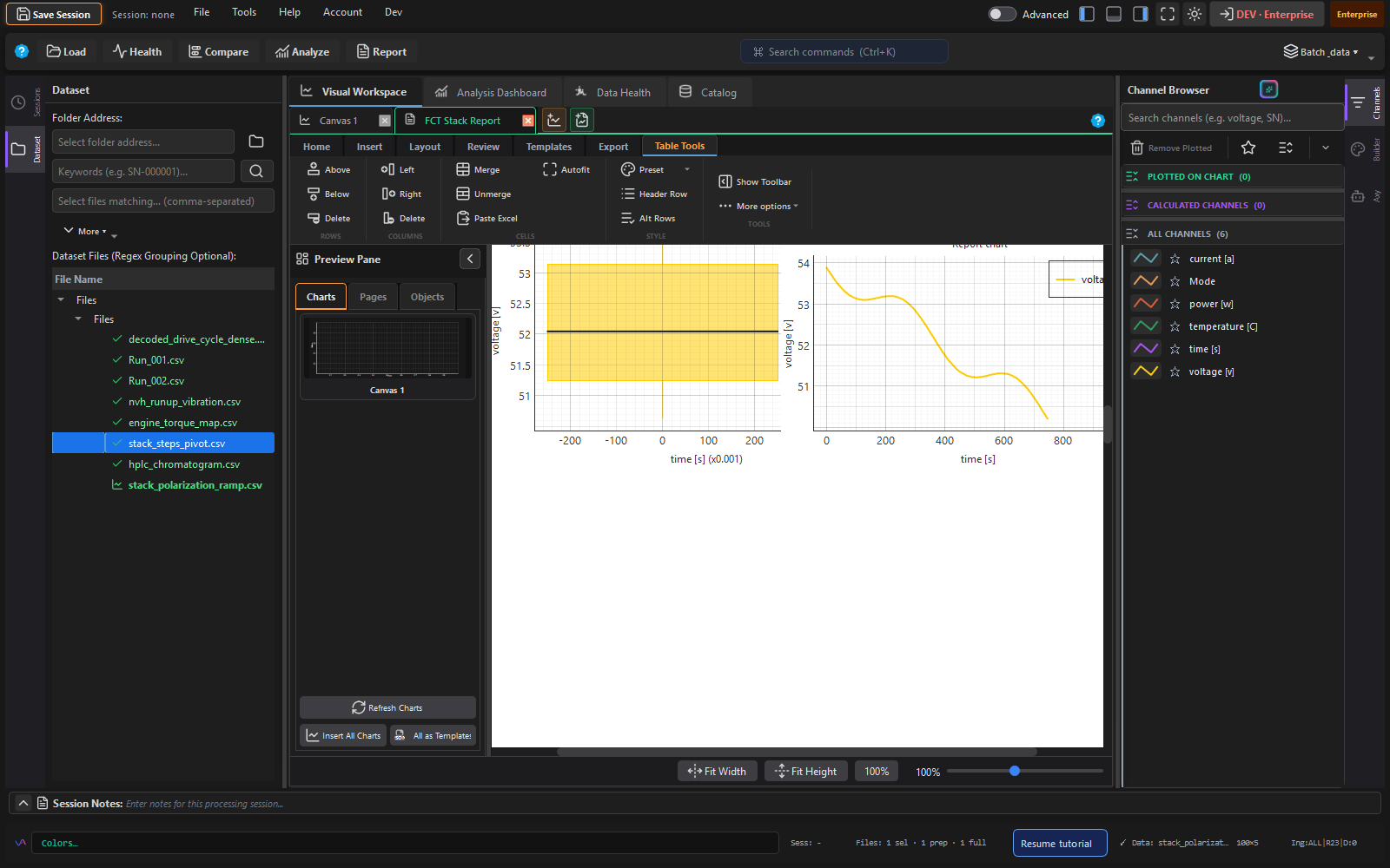
Generate professional PPTX, Word, or PDF reports from reusable templates. Batch-process entire folders. Save pipeline recipes for one-click re-runs on new data.
Power Mode
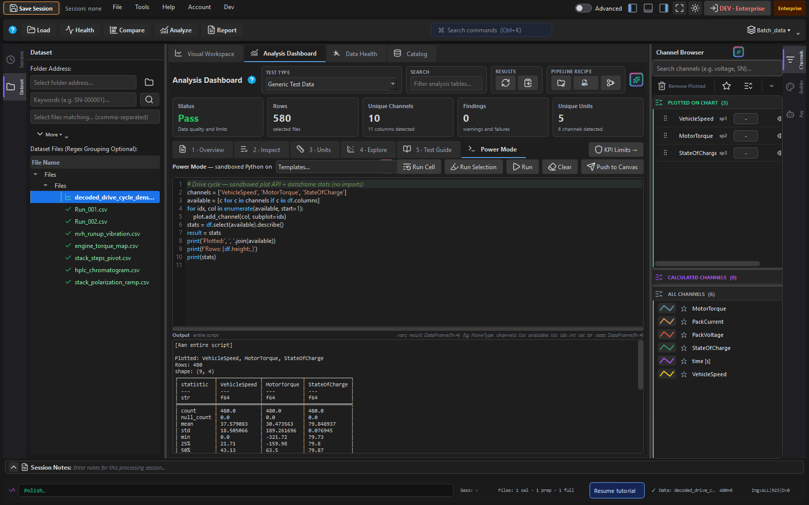
Sandboxed Python against the active canvas dataset - plot scripting, dataframe transforms, and inline stats from the Analysis Dashboard.
- Press F1 for a searchable reference of every chart option, with one-click snippets
- Autocomplete lists every loaded channel and explains each chart option
- Ask Axy to write a script or a reusable function and review it in the editor before saving
Report Template Builder
Accessed from the Report panel or Tools → Report → Template Builder. Design templates with:
- Text blocks with dynamic placeholders (channel values, statistics, localized date/time)
- Auto-populated data tables (stats, limits, delta)
- Chart references (any chart in the current session)
- KPI cards with conditional pass/warn/fail colouring
- ISO 17025-style metadata fields (operator, instrument, calibration date)
- Computed columns and formulas
Templates are saved as .dpt files. Vizalyze ships with three ready-to-use templates for fuel cell stack analysis.
Pipeline DAG & Recipes
The pipeline view lets you wire up processing steps in dependency order:
health_check → compare_runs → limit_eval → analyze → auto_summary → export_pptxSteps run in topological order. Save the full pipeline as a recipe JSON in Recipes/. Load any recipe and re-run it on a new batch of files - ideal for repeated test campaigns.
Workflow Library
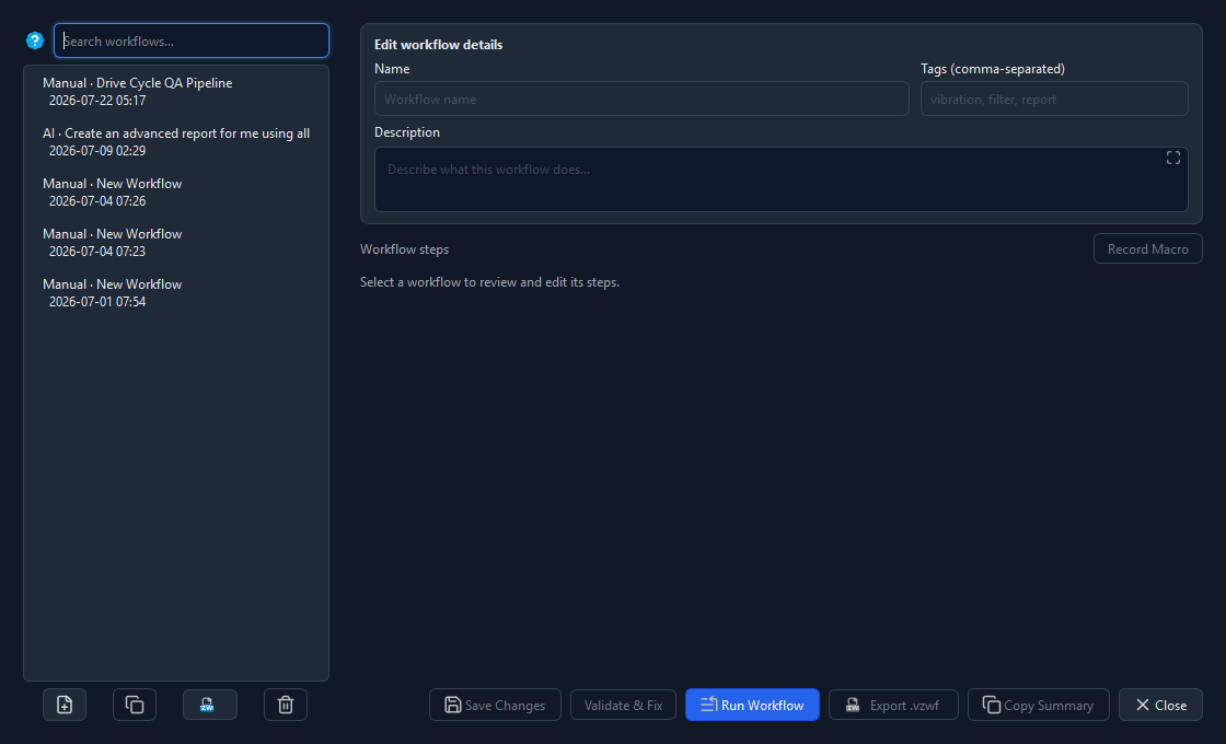
Save AI-assisted or manual analysis sequences as named workflows. Browse, duplicate, export as .vzwf, and replay on new data from Tools → Workflow → Workflow Library.
Auto-summary
The "Auto Summary" feature merges findings from the Data Health and Compare Runs panels into a single narrative section that goes into the report automatically.
7 built-in presets
- Durability report
- Run comparison report
- Sensor drift report
- Step test report
- Limit check report
- Transient response report
- Efficiency analysis report
Chart Types
17 chart types powered by Pyqtgraph with OpenGL acceleration. Every chart is interactive: zoom, pan, hover tooltips, cursor measurement, right-click styling, and legend toggling.
| Chart | Best for | Notes |
|---|---|---|
| Line | Continuous time-series trends | Default for time-indexed data |
| Scatter | Correlation & clustering | Optional trend line overlay |
| Line + Markers | Discrete sample highlighting | Marker shape & size configurable |
| Step Plot | Digital states, relay logic, enums | Horizontal steps at each sample |
| Stacked Subplots | Multi-channel with independent Y-axes | Linked X-axis pan/zoom |
| Bar / Histogram | Grouped comparisons, binned distributions | Grouped, stacked, or auto-binned mode |
| Stacked Bar | Part-of-whole composition | 100% normalised option |
| Waterfall | Cumulative variance bridges | Show absolute or relative deltas |
| Area (Filled) | Magnitude & cumulative emphasis | Stacked area supported |
| Strip Chart | Live feed / scrolling recorder simulation | Configurable history window |
| Run Chart | Segment-by-segment shape comparison | Step-function segments per run |
| Weibull Plot | Reliability & failure rate analysis | Log-log scale, fit line |
| Box Plot | Distribution: median, quartiles, outliers | Outlier points rendered individually |
| 3D Scatter Map | Operating maps, DOE clouds (X/Y/Z) | Viridis colour by Z; rotate in 3D |
| 3D Surface Map | Gridded response surfaces (MATLAB-style) | PyOpenGL; viridis height colouring |
| Heat Map (2D) | Top-down colour-intensity maps | Configurable colour scale |
| Live Cursor Bar | Animated playback scrubbing | Bars update in real-time as cursor moves |
Chart interaction features
- Hover highlighting - active series brightens on mouse-over, others dim
- Click selection - click a series to select it; stats appear in the status bar
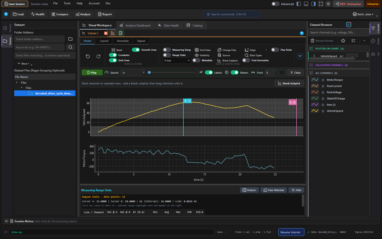
- Inspect tool (A/B cursors) - shaded measuring range with A/B handles; live ΔY / ΔX / 1/ΔX readout and min/avg/max/P2P/std for every plotted channel
- Export - PNG, PDF, SVG from right-click context menu; Copy Chart Image (Ctrl+Shift+C) for PowerPoint / Teams
- Legend - draggable; click series name to toggle visibility
- Per-series styling - colour, line width, dash pattern, marker shape
- Alert bands - define horizontal limit zones with colour fill
Performance
Vizalyze renders 1M+ data points instantly using LTTB (Largest Triangle Three Buckets) peak-preserving downsampling. In Auto mode, downsampling activates automatically for dense signals. In Quality mode, full resolution is kept. See Performance settings below.
Performance & Cache
Vizalyze is engineered for speed on large datasets. Three performance modes let you choose the balance between quality and responsiveness.
Performance modes
- Auto (recommended) - activates optimisations adaptively based on data size
- Quality - preserves full resolution; may be slower on 1M+ point datasets
- Maximum Speed - aggressive optimisations: heavier downsampling, smaller 3D point caps, disabled antialiasing
Auto plot optimisations
- LTTB peak-preserving downsampling (configurable on/off)
- Clip-to-view: only renders points in the current viewport
- Adaptive antialiasing: disables on dense plots, re-enables after zoom
- Marker & label caps: limits number of decorations rendered at once
- 3D scatter point caps: 500k (Quality) / 150k (Auto) / 50k (Max Speed)
- Hover tracking throttle on dense plots
Parquet cache
On first load, CSV and other text formats are automatically converted to Parquet and stored in the Sessions/ folder. Re-opening a cached file is near-instant (Polars lazy scan vs full text parse). Cache is LRU-evicted to manage disk usage.
Performance benchmarks
| Operation | Time |
|---|---|
| Polars eager CSV read (100k rows) | ~357 ms |
| Polars lazy preview (2k rows) | ~22 ms |
| asammdf MDF4 load (100k × 4 ch) | ~130 ms |
| npTDMS TDMS load (100k × 4 ch) | ~25 ms |
| FTS metadata catalog search | ~13 ms |
| Unit conversion (vectorised) | ~300× faster than row-by-row |
| Catalog index update (batched) | ~50× faster than per-file |
Diagnostics
Export a performance log from Help → Diagnostics → Export Performance Log. The log captures timing for startup, file loads, chart redraws, and catalog searches - useful for diagnosing slowdowns on specific hardware.
Enable verbose tracing with the environment variable DPT_PERF_TRACE=1.
Signal Processing
100+ signal processing functions available from the Analysis panel, Code panel, and right-click chart menu. Every result is a computed column with full lineage tracking.
Frequency analysis
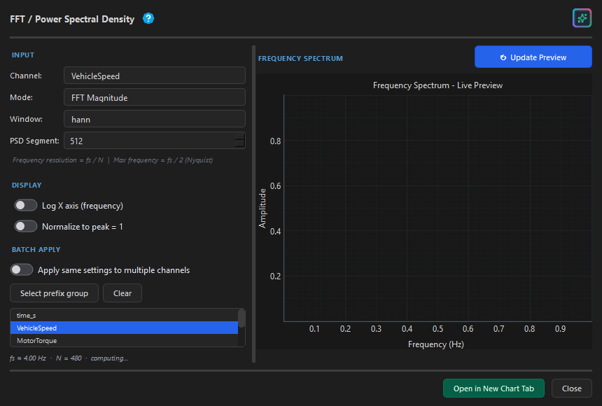
- FFT - Fast Fourier Transform with Hann, Hamming, or Blackman windowing
- PSD - Power Spectral Density using Welch's method
- Spectrogram (STFT) - Short-Time Fourier Transform with log-scaled power display
Digital filtering
- Filter families: Butterworth, Chebyshev I, Chebyshev II, Bessel, Elliptic
- Filter types: Low-pass, High-pass, Band-pass, Band-stop
- Phase mode: Zero-phase forward-backward filtering (no phase delay)
- Order: 1 to 10, configurable
Smoothing
- Moving average (simple, exponential)
- Median filter
- Savitzky-Golay (polynomial smoothing)
Transforms
- Resampling - interpolate to a uniform time grid at any target rate
- Differentiation - numerical first and second derivatives
- Integration - cumulative numerical integration (trapezoid rule)
- Unit conversion - vectorised affine transforms (~300× faster than row-by-row)
Event detection
- Peak detection - configurable minimum height and distance
- Anomaly detection - statistical outlier flagging (z-score, IQR)
- Step detection - identify step changes and segment by state
NVH & durability
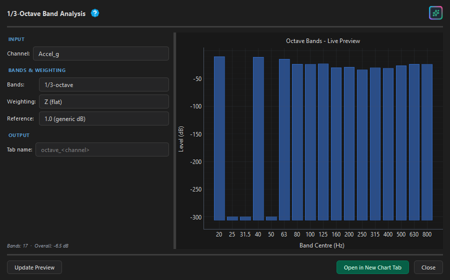
- 1/3-Octave bands - IEC 61260 fractional-octave levels with A/C/Z weighting and optional 20 µPa SPL reference
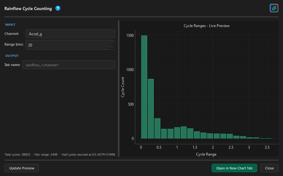
- Rainflow counting - ASTM E1049 cycle ranges and histogram for fatigue / S-N damage models
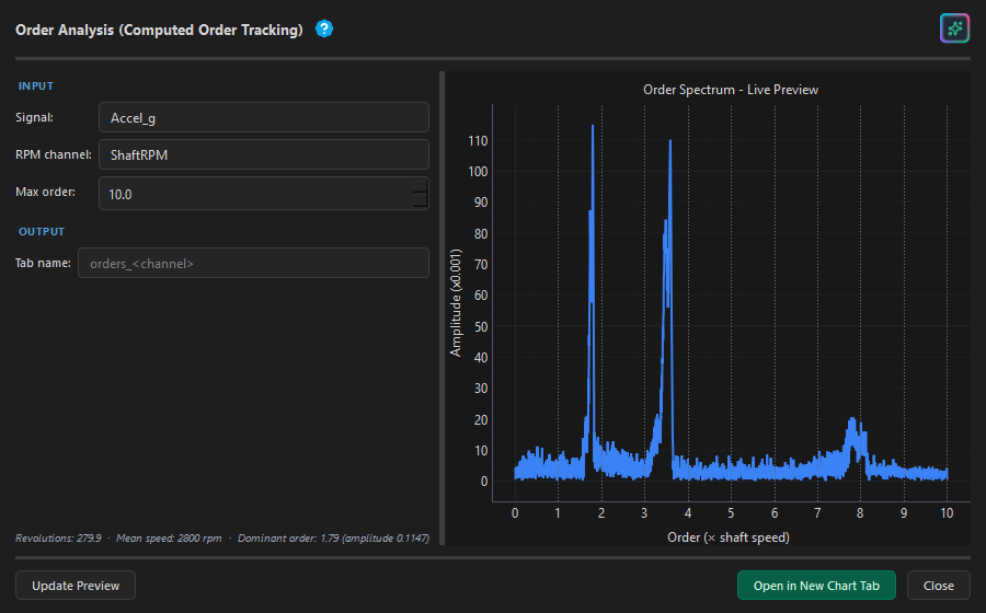
- Order analysis - computed order tracking via angular resampling against an RPM channel
Pivot / Group-By
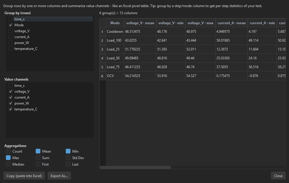
Summarise any loaded dataset like an Excel pivot table: group by mode/step columns, aggregate channels (mean/min/max/sum/std/…), then copy as TSV or export. Open from Tools → Data → Pivot / Group-By Summary or the command palette.
Custom Functions
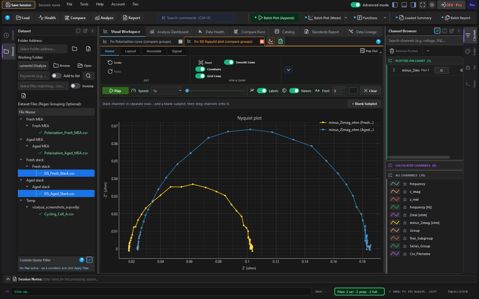
Save any Power Mode script as a reusable function with its own run form, run it on any selection of files, and compare groups on one chart. A library of standards-based functions for electrochemistry, battery and EV, emissions, durability, statistics and stability testing is included with the domain packs.
Read the Custom Functions guide →
Code Panel
Write Python-syntax expressions to add computed columns or filter rows - directly in the app, with AI autocomplete and inline error messages.
Computed columns
# Example: compute power from voltage and current
Power_kW = (HV_Voltage * HV_Current) / 1000

# Example: efficiency ratio
Efficiency = Motor_Power_out / Motor_Power_in
Column names auto-complete as you type. Available functions include Polars expressions, numpy operations, and all custom transforms.
Filter conditions
# Keep only rows where vehicle is moving above 5 km/h
Vehicle_Speed > 5

# Keep rows in a specific temperature range
(Battery_Temp >= 15) & (Battery_Temp <= 40)
Filter conditions create a new derived dataset - the original data is untouched (immutable lineage). Toggle the filter on/off in the dataset tree.
AI assistance
Click the AI button (or type /ai) in the code panel to describe what you want in plain English. The AI generates the expression using your actual column names and explains its reasoning.
Metadata Catalog
An FTS5 SQL-backed searchable index of all files Vizalyze has ever seen. Stays fast with 50,000+ indexed files.
What gets indexed
- File path, format, size, modification date
- Row count, channel count, time column name
- Column names (all, searchable as full-text)
- Health status (Pass/Warn/Fail)
- Test ID and run ID (parsed from preamble)
Search filters
- Full-text search across column names and file paths
- Format filter (by extension)
- Date range picker
- Health status filter
- "Discovered only" - files seen but not loaded
Double-click any result to load it into the active session. The catalog updates in the background when the working folder changes. Files whose mtime hasn't changed reuse cached metadata (no re-read needed).
Data Lineage & Provenance
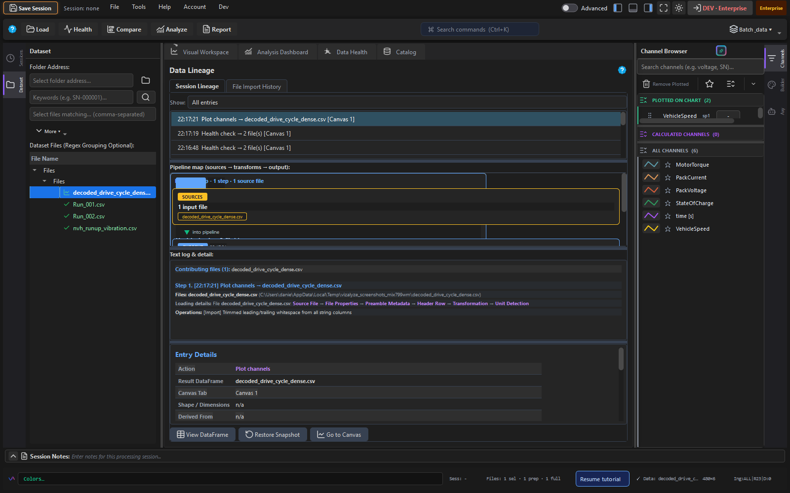
Every load, filter, merge, transform, and computed column is tracked in an immutable dependency graph.
Data Lineage Panel
Visualise the full transformation DAG - see exactly how each dataset was derived. Each node shows the operation, timestamp, and operator (on Team tier).
Rollback
Revert to any prior state in the workflow by clicking a node in the lineage graph. The original file is never modified.
Audit log (Team+)
Append-only, immutable audit log records every action: who loaded which file, when, what transforms were applied, and what was exported. Meets requirements for regulated environments.
Automotive & CAN/LIN
Native support for ASAM MDF files and CAN/LIN bus decoding. The Automotive & EV extension pack includes:
Supported MDF formats
.mf4- ASAM MDF4 (all versions, current standard).mf3- ASAM MDF3 (legacy).mf2- ASAM MDF2 (legacy).atfx- ASAM ODS Transfer Format
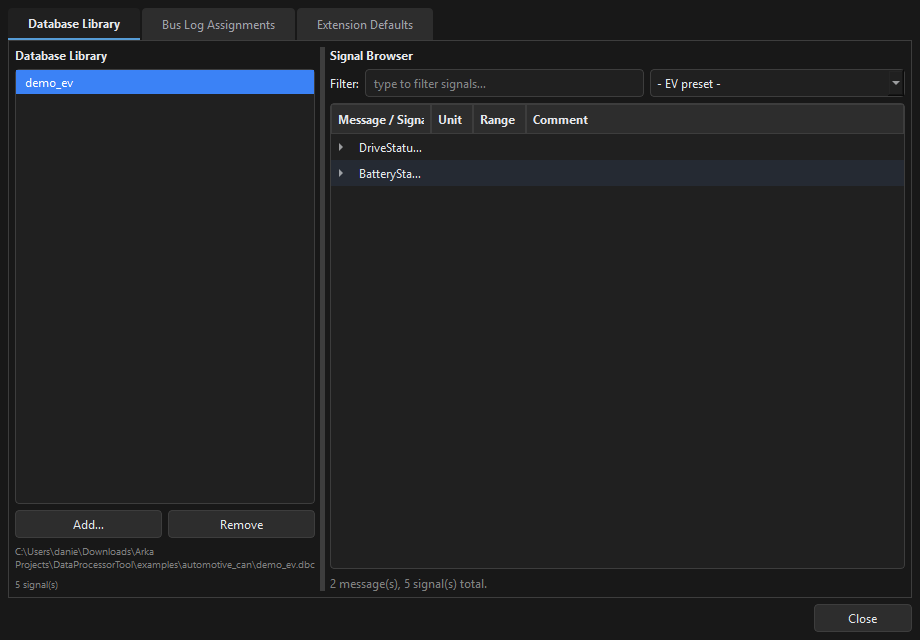
CAN Database Manager
Open from Tools → Data → CAN Database Manager. Features:
- Persistent library of DBC, ARXML, KCD, SYM database files
- Browse message/signal trees with IDs, units, min/max, factor, offset, comments
- Free-text search across all signal names and descriptions
- Assign a database to a specific file, or set as the global default
- 6 built-in EV signal presets (see below)
EV signal presets
| Preset | Included channels |
|---|---|
ev_speed | Vehicle & wheel speed, RPM, odometer |
ev_torque | Motor & drivetrain torque (request and actual) |
ev_battery | HV voltage, current, SOC, cell voltages |
ev_temperature | Battery, motor, inverter, coolant temperatures |
ev_driver | Throttle pedal, brake pedal, steering angle, gear selector |
ev_drive_cycle | All of the above - complete drive cycle snapshot |
Automatic CAN decoding
When a database is assigned (via the CAN Database Manager or an import template), CAN/LIN signals are decoded automatically on load. MDF/MF4 files use asammdf.MDF.extract_bus_logging(); BLF files use python-can + cantools. Physical signals (with scaling applied) appear directly as columns in both cases.
BLF (Vector Binary Log) support - new in v1.0.7
Vector .blf captures are now a first-class format. Drop a BLF file into the Files panel like any other source. Two modes:
- Without DBC assigned - raw frame inspection:
timestamp,arbitration_id,dlc,data_hex. Useful to verify what message IDs are present before assigning a database. - With DBC/ARXML assigned - full signal decode: open the CAN Database Manager (Tools - Data - CAN Database Manager), pick your BLF file under Bus Log Assignments, assign the matching database, then reload. Every signal appears as its own named column with physical units.
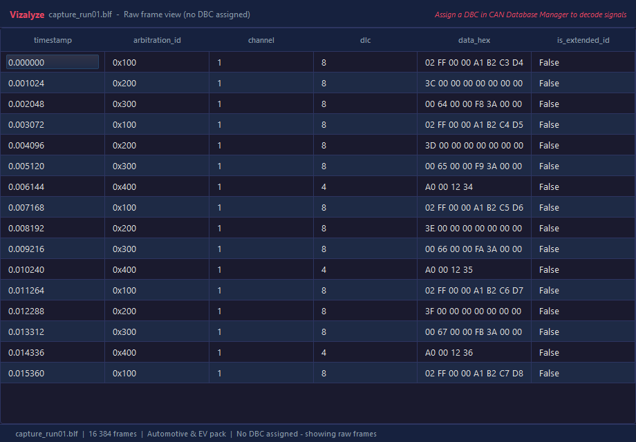
BLF loaded without a DBC: raw frame columns for quick inspection of message IDs and payloads.
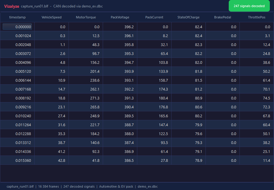
Same BLF file after assigning vehicle.dbc: 247 signals decoded into named, scaled columns.
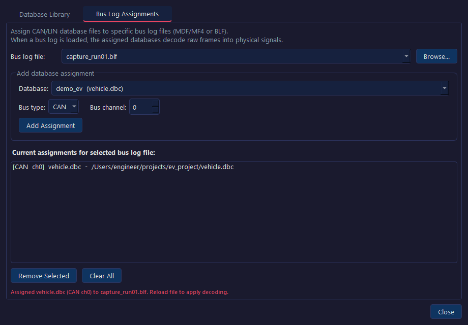
The Bus Log Assignments tab accepts BLF and MDF/MF4 files. Select your file, pick a database from the library, and click Add Assignment.
The same DBC library and assignment workflow used for MDF/MF4 files applies unchanged to BLF - no extra setup required if you already have databases configured.
Export Dataset As - new in v1.0.7
Any loaded or processed dataset can be exported to a portable format via Tools - Data - Export Dataset As.... This works on all ingested formats: BLF decoded signals, MDF/MF4, TDMS, HDF5, NetCDF, and all others.
- CSV / TSV - universally readable, works in Excel, Python, R
- Excel (.xlsx) - formatted workbook for sharing with stakeholders
- Parquet - compressed columnar format for large datasets (zstd compression)
- Feather / Arrow IPC - zero-copy interchange with pandas, polars, R Arrow
- JSON - row-oriented JSON for web and API consumers
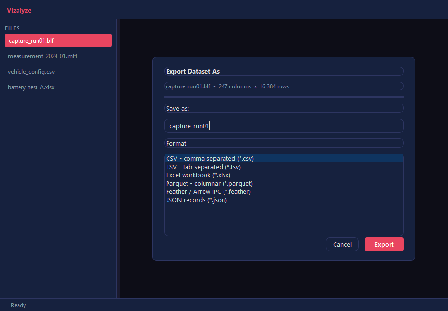
Export any loaded dataset - including decoded BLF signals - to CSV, Excel, Parquet, Feather, or JSON in one click.
Pharma & Analytical Chemistry
The Pharma extension pack provides native support for the most common analytical chemistry data formats, plus domain-specific analysis profiles.
Supported formats
- .cdf - AIA/ANDI CDF chromatography data (netCDF-based). Columns:
retention_time,signal. Supports HPLC, GC, IC. - .mzml - mzML mass spectrometry. Extracts TIC (Total Ion Current), BPI (Base Peak Intensity), and per-scan summaries. Requires
pymzml. - .jdx / .dx - JCAMP-DX spectra and chromatograms. Supports NMR, IR, UV-Vis, Raman, mass spectra. Columns: numeric X/Y.
- .raw - Thermo Fisher RAW files. Requires external ThermoRawFileParser converter (free, open-source).
- .wiff - Sciex WIFF files. Requires external ProteoWizard
msconvert(free).
Pharma domain profiles
- Pharma HPLC - retention time, peak area, resolution, symmetry factor, tailing factor, theoretical plates
- Pharma GC - peak area %, relative retention time, split ratio diagnostics
- Pharma MS - TIC, BPI, spectral purity, fragment ion ratios, m/z ranges
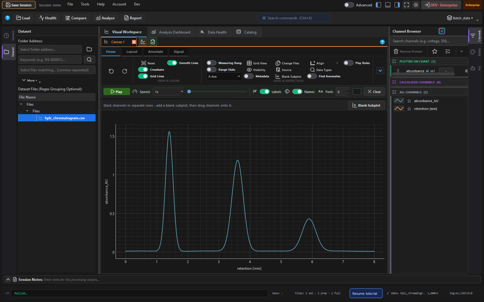
ISO 17025-style metadata and traceability fields
Report templates include ISO 17025-style metadata fields: analyst name, instrument serial, calibration date, method reference, and sample ID. These populate automatically from preamble metadata when detected.
File-based live tailing & SPC
Tail measurement files as they grow on disk (not a hardware DAQ stream). Mark any supported file as a live source — Vizalyze polls for appends and updates the chart automatically.
Setup
- Right-click a dataset in the file tree → Mark as live source
- Set the poll interval in Settings → Performance & Cache (default: 2.0s; range 250ms–10s)
- The chart and statistics refresh when new rows are appended to the file
Live SPC panel
- Control-limit style monitoring (UCL, LCL, warning limits)
- Real-time plot & statistics refresh
- Drift detection and out-of-control rule alerts
- Alarm annotations on the chart
examples/live_monitoring/ folder includes a 3-minute demo with a sample live CSV and an append_rows.py script that simulates a live instrument feed.AI Integration
Vizalyze has a built-in AI chat panel and AI-assisted features throughout the app. All AI calls go directly to your chosen provider - Vizalyze is never the intermediary.
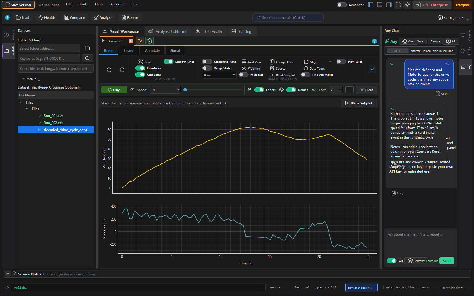
Built-in AI chat panel
Ask questions about your loaded data in plain English. The AI has access to your column names, statistics, and health report. Example queries:
- "Which channel shows the highest correlation with Battery_Temp?"
- "Write a Butterworth low-pass filter at 5 Hz for the Vibration_Z channel"
- "Summarise the key findings from the data health report"
- "Generate a report recipe that compares Run_001 and Run_002 on speed and SOC"
AI-assisted features
- Code panel - describe a computed column or filter condition in English; AI generates the Polars expression
- Chart styling - "make the speed line red and the SOC line dashed green"
- Channel recommendations - AI suggests which channels to plot based on data health findings
- Formula autocomplete - intelligent suggestion of channel names and operators as you type
Supported providers
- Claude (Anthropic) - recommended for analytical reasoning
- GPT-4 (OpenAI) - broad capability
- Gemini (Google) - fast responses
- Ollama - fully local, no data leaves the machine
- LM Studio - fully local with a GUI model manager
Configure your API key in Control Settings → AI. For local models, set the server URL (default http://localhost:11434 for Ollama).
AI Environments (Pro+)
Save and restore AI conversation context to the cloud. Switch machines and pick up exactly where you left off - the AI remembers your project context, preferred channel names, and analysis conventions.
Files, Tabs & Reports
Vizalyze keeps three things separate, so you always know which files feed which chart or report.
- Loaded files - the files in the Dataset panel that are in memory. Only Load and Unload change this.
- Tab sources - the files each chart tab was built from. Plot Details lists them with a status: Loaded, Changed on disk, Not loaded or Snapshot.
- Tree selection - the files you highlight. Selecting or deselecting never changes a tab; it only chooses what Update This Tab or Plot on New Tab will use.
What happens when...
- You deselect a file - nothing changes in any tab or report.
- You add a file - it joins the list and is not used anywhere until you plot it.
- You switch tabs - each tab keeps its own files. In the Dataset tree, files used by the open tab are highlighted brightly and files only other tabs use are muted. Hover a file, or right-click and choose Where is this used?, to see its tabs and reports.
- You unload a file that other tabs use - Vizalyze asks first. Keep as snapshot (the default) lets those tabs keep the data they show without following the file. Remove from those tabs rebuilds them without it.
- You use Remove from List - only the list entry goes away. The data stays loaded and nothing is deleted from disk.
- Data changes in a tab - reports show which tab changed. Refresh redraws each chart from the tab it was made from.
- You freeze a report chart - right-click it and choose Freeze data. Refresh skips it.
- You save and reopen a session - tabs reload their files from disk. Snapshots last only for the current session.
Sessions
Sessions save the complete state of a Vizalyze project: loaded files, charts, filters, computed columns, compare settings, analysis results, and AI conversation context.
Save & load
Sessions are stored in Sessions/ inside your working folder. Use File → Save Session or Ctrl+S. On startup, Vizalyze can auto-restore the last session (configurable: Always / Ask / Never).
Each canvas keeps its own Multi-Y, Shared X, Markers, Legends, Log scale, Grid, Crosshair and Anti-aliasing switches, and Resume from the welcome screen reloads the session's files so charts and reports come back.
Session limits
- Free - local sessions only, unlimited
- Pro - 25 cloud-synced sessions
- Team - 200 cloud-synced sessions
Cloud Features (Pro+)
Desktop vs website: Analysis always runs in the installed app. Cloud features sync settings from the desktop and expose a few read-only experiences on vizalyze.app (account dashboard, shared report viewer, live monitor). Raw measurement files are not uploaded for analysis in the browser.
Encrypted cloud sync
Workflows, sessions, templates, and channel configs are encrypted with AES-256-GCM before leaving your machine. Your encryption key is derived from your credentials - Vizalyze's servers never have access to your content.
Secure report sharing
From the desktop app, publish a report and generate a share link. Recipients open an interactive read-only view in their browser at vizalyze.app - no desktop install required. Links can be set to expire.
Live monitor dashboard (web)
Pro+ users can open a browser dashboard on vizalyze.app to watch live statistics and sparklines for files the desktop app is monitoring - a companion view, not a substitute for the desktop Visual Workspace.
Org workspace (Team+)
Shared workspace with org-scoped template library, channel config library, and CAN database library. All members see the same shared resources.
Settings & Configuration
Access all settings from the Control Settings step in the ribbon, or from the ⚙ icon in the top-right.
| Category | Options |
|---|---|
| Working Folder | Choose project directory; subdirectories auto-created |
| UI Mode | Basic (curated core tabs) | Advanced (all tabs visible) |
| Performance Mode | Auto | Quality | Maximum Speed |
| Plot Auto-Optimise | On / Off (downsampling, clip-to-view) |
| Channel Cleanup | Per-format regex replacement rules (enable/disable) |
| CSV Preamble | Mode, delimiter, number of header rows |
| Unit Detection | From metadata | From header row | Scan N rows |
| Excel Sheet Policy | Load first | Load all | Prompt each time |
| Session Restore | Always | Ask on startup | Never |
| AI Provider | Provider, API key, local model URL, model ID |
| CAN Database Library | Add/remove databases and assignments |
| Chart Styles | Save custom presets (background, grid, axis colours) |
Machine-level settings
Stored in ~/.Vizalyze/app_settings.json. This includes your working folder path, performance mode, and API keys (encrypted).
Environment variables
DPT_PERF_TRACE=1- verbose performance tracing to stderrVIZALYZE_DEV=1- enable developer mode (unlocks all tiers locally)QT_QPA_PLATFORM=offscreen- headless mode for CI/automated testing